Google Sheets is a powerful tool for organizing and analyzing data. It offers a wide range of features and functions to make working with spreadsheets easier and more efficient. One of the key functions that can be used in Google Sheets is the text function. In this guide, we will dive into 15 simple Google Sheets text functions that you can use to manipulate and analyze text in your spreadsheets.
Overview of Google Sheets Text Functions
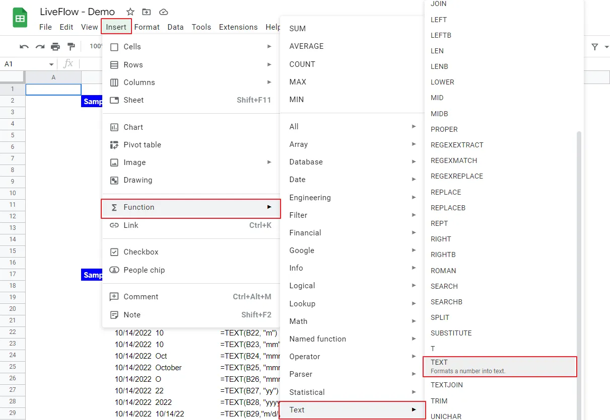
Before we delve into the specific text functions, let’s first understand what they are and how they work. Text functions in Google Sheets are formulas that allow you to perform various operations on text strings. These operations include manipulating, splitting, combining, and searching for text within a cell or range of cells. These functions are especially useful when dealing with large amounts of data, as they can save you time and effort from manually performing these tasks.
Now, without further ado, let’s explore some of the most valuable Google Sheets text functions that you can start using today.
1. CONCATENATE Function
The CONCATENATE function in Google Sheets allows you to combine multiple text strings into one cell. This can be useful when merging first and last names, addresses, or any other pieces of text. The syntax for this function is straightforward – =CONCATENATE (text1, text2, …). You can add up to 30 text strings within the parentheses, separated by a comma.
Example:
Consider the following data in a Google Sheet:
| Column A | Column B |
|---|---|
| John | Doe |
| Jane | Smith |
To combine the first name and last name into one cell, we can use the formula =CONCATENATE(A2,” “,B2) in column C. This will result in “John Doe” in cell C2 and “Jane Smith” in cell C3.
2. UPPER, LOWER, and PROPER Functions
The UPPER, LOWER, and PROPER functions are all used to change the case of text strings in Google Sheets. The UPPER function converts all letters to uppercase, the LOWER function converts all letters to lowercase, and the PROPER function capitalizes the first letter of each word while converting the rest to lowercase. These functions can be useful when you need to standardize the case of data or when manipulating names or titles.
Example:
Let’s use the same data from our previous example. In column D, we can apply the UPPER, LOWER, and PROPER functions to convert the names in column A to uppercase, lowercase, and proper case, respectively. The formulas would be =UPPER(A2), =LOWER(A2), and =PROPER(A2). This will result in “JOHN”, “john”, and “John” in cells D2, D3, and D4, respectively.
3. LEFT, RIGHT, and MID Functions
The LEFT, RIGHT, and MID functions allow you to extract a specific number of characters from the beginning (LEFT), end (RIGHT), or middle (MID) of a text string. These functions can be handy when working with data that has consistent formatting, and you want to isolate certain parts of it.
Example:
Let’s say we have a list of email addresses in column E, and we want to extract only the domain name (the part after the “@” symbol). We can use the MID function to do this by specifying the start character as the position of the “@” symbol plus one. The formula would be =MID(E2,FIND(“@”,E2)+1,LEN(E2)). This will return “gmail.com” from the email address in cell E2.
4. LEN and TRIM Functions

The LEN function is used to determine the length of a text string in a cell. This can be useful when you need to check if data meets certain length requirements, such as a password or a phone number. The TRIM function, on the other hand, removes any leading or trailing spaces from a text string. This is particularly helpful when dealing with data that has inconsistent spacing.
Example:
In column F, we have a list of phone numbers with varying lengths and some unnecessary spaces. To determine which numbers are less than 10 digits, we can use the LEN function and set up a conditional formatting rule that highlights cells with values below 10. Additionally, we can use the TRIM function in column G to remove any extra spaces from the phone numbers.
5. FIND and SEARCH Functions
The FIND and SEARCH functions are used to locate a specific text within a larger text string. The difference between them is that FIND is case-sensitive, while SEARCH is not. Both functions return the position of the first character of the text being searched for. If the text is not found, both functions return an error.
Example:
Let’s say we have a list of URLs in column H, and we want to extract only the domain name (the part after “www.”). We can use the FIND function to locate the position of the “.” after “www.” and then use the RIGHT function to extract everything after it. The formula would be =RIGHT(H2,LEN-FIND(“.”,H2,FIND(“www.”,H2))). This will return “example.com” from the URL in cell H2.
6. SUBSTITUTE Function
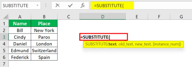
The SUBSTITUTE function allows you to replace a specific text within a cell with a new text. This can be useful when correcting spelling errors or changing formatting. You can also specify which instance of the text you want to substitute, in case there are multiple occurrences within the cell.
Example:
Let’s say we have a list of product codes in column I, but they all have an extra “0” at the end that needs to be removed. We can use the SUBSTITUTE function to replace the last “0” with an empty string “”. The formula would be =SUBSTITUTE(I2,”0″,””,LEN(I2)-1). This will return the corrected product code without the extra “0”.
Conclusion
Google Sheets text functions are essential for manipulating and analyzing data in spreadsheets. They can save you time and effort by automating tasks that would otherwise be done manually. In this guide, we covered some of the most useful and simple text functions that you can start using today. With these functions, you can now take your data analysis skills to the next level.