Google Sheets is a powerful spreadsheet software that allows users to organize data, create charts and graphs, and collaborate with others in real-time. With its user-friendly interface, it has become a popular choice for individuals and businesses alike. One useful feature of Google Sheets is the ability to highlight texts, which can make data easier to read and interpret. In this article, we will explore different ways on how to highlight texts in Google Sheets manually and automatically.

Manual Highlighting in Google Sheets

Using the Fill Color Tool

The simplest way to highlight text in Google Sheets is by using the “Fill Color” tool. To do this, follow these steps:

1. Select the cell or cells you want to highlight.
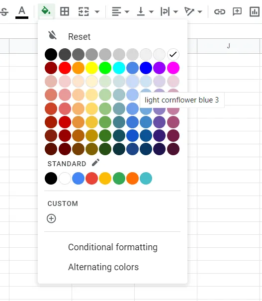
2. Click on the “Fill Color” icon on the toolbar, which looks like a paint bucket.
3. A drop-down menu will appear with a variety of colors to choose from. Select the color you want for your highlight.
4. The selected cells will now be highlighted with the chosen color.

You can also access the “Fill Color” tool by right-clicking on the selected cells and choosing “Fill color” from the menu.

Using Conditional Formatting

Another way to manually highlight texts in Google Sheets is by using the “Conditional Formatting” feature. This allows you to automatically apply formatting based on certain conditions. To use this feature, follow these steps:

1. Select the cells you want to apply conditional formatting to.
2. Click on the “Format” tab on the toolbar and select “Conditional formatting” from the drop-down menu.
3. In the side panel that appears, click on the drop-down menu next to “Format cells if” and choose “Custom formula is.”
4. In the box below, enter the criteria that must be met for the cells to be highlighted. For example, if you want to highlight cells that contain the word “Sales,” you can enter the formula
   =SEARCH(“Sales”, A1)>0

   , assuming that the cell you want to check is A1.

5. Choose the formatting style you want to apply by clicking on the paint bucket icon next to “Format cells.” You can also choose the fill color, text color, font style, and more.
6. Click on “Done” and the cells that meet the criteria will be automatically highlighted.

You can also add multiple conditions by clicking on the “+” button in the side panel. This allows you to create more complex rules for highlighting texts in Google Sheets.

Using the Format Painter Tool

The “Format Painter” tool is a useful feature in Google Sheets that allows you to quickly copy formatting from one cell or range of cells to another. To use this tool for highlighting texts, follow these steps:

1. Select the cell or range of cells with the formatting you want to copy.
2. Click on the “Format Painter” tool on the toolbar, which looks like a paintbrush.
3. The cursor will change into a paintbrush icon. Click on the cell or cells you want to apply the formatting to, and it will be automatically copied.
4. To turn off the “Format Painter,” click on the tool again or press the “Esc” key on your keyboard.

Automatic Highlighting in Google Sheets

Using Conditional Formatting with Custom Formulas

As mentioned earlier, conditional formatting can be used to automatically highlight texts in Google Sheets. However, instead of using the built-in options, you can create custom formulas to apply more specific conditions. Here are some examples of custom formulas you can use for automatic highlighting:

• Highlight duplicates:
  =COUNTIF($A$1:$A, A1)>1

  – this formula will highlight all duplicate values in column A.

• Highlight values above or below a certain threshold:
  =A1>100

  – this formula will highlight all values in column A that are greater than 100.

• Highlight cells with specific text:
  =SEARCH(“Sales”, A1)>0

  – this formula will highlight all cells in column A that contain the word “Sales.”

You can adjust the formulas according to your own data and criteria. The key is to use the correct syntax and logical operators to create the desired result.

Using Data Bars

Data bars are a great way to visually represent data in Google Sheets. They add a colored bar to each cell, which corresponds to the value in that cell. This makes it easy to identify high or low values at a glance. To use data bars for highlighting texts, follow these steps:

1. Select the cell or range of cells you want to apply data bars to.
2. Click on the “Format” tab on the toolbar and select “Conditional formatting” from the drop-down menu.
3. In the side panel that appears, click on the drop-down menu next to “Format cells if” and choose “Greater than.”
4. In the box below, enter the threshold value. For example, if you want to highlight values greater than 100, enter the number 100.
5. Choose the formatting style you want to apply by clicking on the paint bucket icon next to “Format cells.” You can also choose the color, bar type, and more.
6. Click on “Done” and the cells that meet the criteria will be automatically highlighted with data bars.

Using Color Scales

Color scales are similar to data bars, except they use different shades of colors instead of bars. They can be useful for highlighting texts in a gradient based on their values. To use color scales for automatic highlighting, follow these steps:

1. Select the cell or range of cells you want to apply color scales to.
2. Click on the “Format” tab on the toolbar and select “Conditional formatting” from the drop-down menu.
3. In the side panel that appears, click on the drop-down menu next to “Format cells if” and choose “Greater than or less than.”
4. In the box below, enter the threshold values. For example, if you want cells with values greater than 100 to be highlighted in red and cells with values less than 50 to be highlighted in green, enter 100 and 50 respectively.
5. Choose the formatting style you want to apply by clicking on the paint bucket icon next to “Format cells.” You can also choose the color scale type and more.
6. Click on “Done” and the cells that meet the criteria will be automatically highlighted with color scales.

Tips and Tricks for Highlighting Texts in Google Sheets

Now that you know how to manually and automatically highlight texts in Google Sheets, here are some additional tips and tricks you can use to make the process even more efficient:

• Instead of selecting each cell individually, you can quickly highlight a large range of cells by clicking on the first cell and then holding down the “Shift” key while clicking on the last cell.
• To select non-consecutive cells, hold down the “Ctrl” key (or “Command” key for Mac) while clicking on each cell.
• You can change the color of the highlighting in the “Conditional formatting” side panel by clicking on the paint bucket icon next to “Format cells.” This allows you to customize the colors according to your preferences.
• If you want to remove the highlighting from specific cells, simply select those cells and click on the “Clear formatting” tool on the toolbar, which looks like an eraser.
• You can copy conditional formatting rules from one set of cells to another by using the “Copy” and “Paste special” options. This is useful if you want to apply the same formatting to different sets of cells.

Conclusion

Highlighting texts in Google Sheets can be done manually or automatically, depending on your needs. The “Fill Color” tool and “Format Painter” tool are quick ways to highlight cells with a specific color, while conditional formatting allows for more customization. By using custom formulas, data bars, and color scales, you can easily highlight texts based on your own criteria. With these tips and tricks, you can make your data more visually appealing and easier to analyze in Google Sheets.